
Suppose I show a language model the word otter, then the word hammer. A neural network turns each input into layers of numbers. Training adjusts millions of connections between those numbers until useful internal responses emerge. You can picture each response as a tiny knob: quiet for some inputs, active for others. I went looking for a knob that seemed to say, “that’s an animal.”
Have we found an animal neuron?
Why expect such a knob at all? Brain studies have found cells and regions that respond selectively to edges, places, faces, and other recurring patterns. Artificial neural networks also learn selective internal responses, although a concept can be spread across many units and one unit can take part in many concepts. The brain analogy gives us a question, not an answer.
That leaves several possibilities. Maybe the unit responds to animals. Maybe it responds to living things, to these particular words, or to some mixture of features. Or maybe a search across enough units will always find an impressive accident.
I built five small experiments in google/gemma-3-1b-pt to separate those possibilities. The first result repeated on new words. The later experiments showed both what that response could reveal and where the story became too simple.
You can play with the recorded responses before reading on. Start with layer 12, unit 646. Then find a unit that prefers plants. The change is a good introduction to the problem.
A familiar idea from psychology
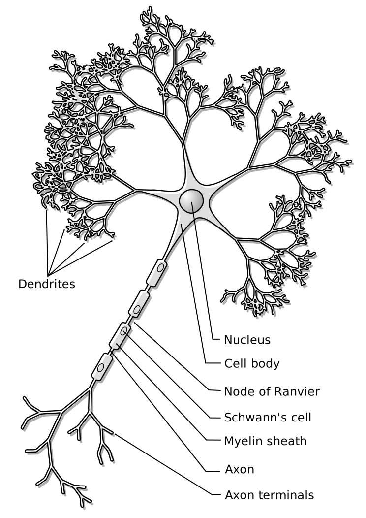
My background is in psychology, so the idea of using a task to locate a response feels familiar. In neuroscience, a functional localizer identifies a region through what it responds to. A classic example compares responses to faces and other objects. Language localizers use contrasts such as sentences versus nonword strings. The details differ, but the useful habit is to locate a response first, then test its properties with independent material. Kanwisher, McDermott, and Chun (1997); Fedorenko et al. (2010).
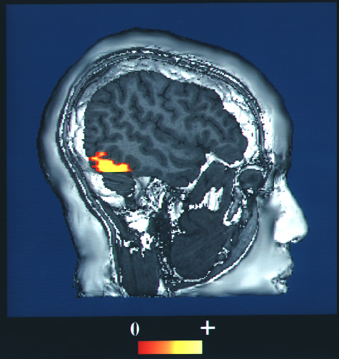
I borrowed that experimental move, not the brain anatomy. An fMRI signal and a model activation are different measurements in different systems. The shared idea is a contrast: find a response with one set of examples, then ask what it does with new examples.
The separation between finding and testing is the part that matters. If I choose a unit because it responds strongly to my animal words, those same words cannot provide an independent test of the result.
First, find a response
The first experiment used 120 words: 60 animals and 60 tools. Every target was one model token, placed in the same sentence:
They mentioned the word {TARGET}For each sentence, I recorded the model’s activations at the position of the target word. I focused on the MLP block: the part of each transformer layer that expands the current representation, applies thousands of nonlinear gates, and compresses it again. MLPs are a natural place to look because research suggests that transformer feed-forward blocks help store and retrieve factual associations. Grant Sanderson gives a visual account of this hypothesis in 3Blue1Brown’s How might LLMs store facts?. It remains a hypothesis about a complicated system, not a promise that one fact lives in one unit.
I recorded the gated MLP intermediate just before it was projected back into the model’s main representation. Gemma has 26 layers and 6,912 such units in each layer. That gave me 179,712 activation knobs to inspect.
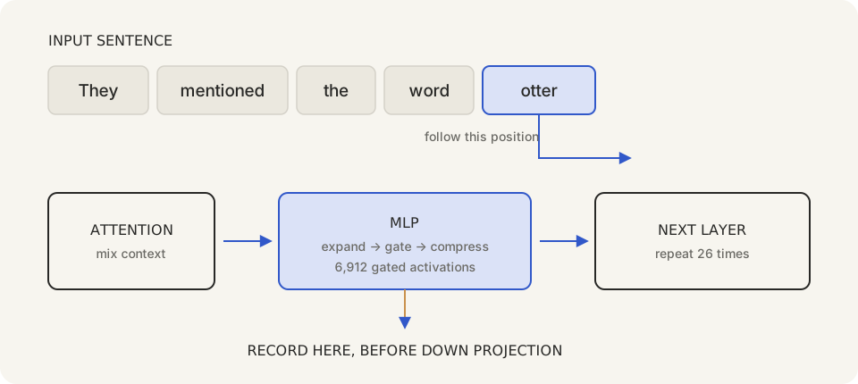
I used 80 words to find units: 40 animals and 40 tools. The other 40 words stayed out of selection. For each unit, I calculated Cohen’s d: the difference between its mean animal and tool responses, divided by the pooled standard deviation.
d = \frac{\text{mean animal response} - \text{mean tool response}}{\text{pooled standard deviation}}
A positive value means the unit responds more to the animal words, relative to the spread of responses. It does not tell us why.
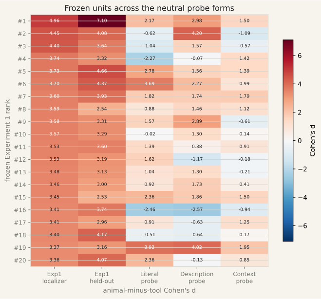
The strongest discovery result was layer 12, unit 646, with d = 4.96. I froze the top 20 unit IDs, then evaluated them on the untouched words. All 20 retained a positive effect; the median held-out d was 3.46. The top discovery unit reached 7.10 on the held-out words. These are large differences for this particular contrast.
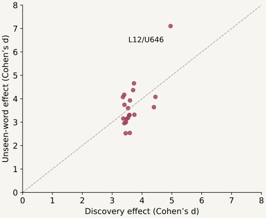
See all 20 selected units
| Rank | Layer | Unit index | Discovery d | Held-out d |
|---|---|---|---|---|
| 1 | 12 | 646 | 4.956 | 7.104 |
| 2 | 17 | 348 | 4.450 | 4.080 |
| 3 | 10 | 5552 | 4.399 | 3.640 |
| 4 | 12 | 1000 | 3.744 | 3.317 |
| 5 | 5 | 1208 | 3.732 | 4.659 |
| 6 | 5 | 2799 | 3.703 | 4.368 |
| 7 | 12 | 4850 | 3.597 | 3.928 |
| 8 | 7 | 3908 | 3.591 | 2.542 |
| 9 | 8 | 3330 | 3.580 | 3.308 |
| 10 | 13 | 3181 | 3.568 | 3.293 |
| 11 | 7 | 6793 | 3.535 | 3.598 |
| 12 | 9 | 4088 | 3.534 | 3.185 |
| 13 | 9 | 3757 | 3.480 | 3.133 |
| 14 | 14 | 971 | 3.461 | 2.996 |
| 15 | 14 | 36 | 3.451 | 2.526 |
| 16 | 9 | 3357 | 3.412 | 3.743 |
| 17 | 13 | 2865 | 3.408 | 2.955 |
| 18 | 7 | 6840 | 3.405 | 4.172 |
| 19 | 13 | 5008 | 3.372 | 3.156 |
| 20 | 8 | 44 | 3.361 | 4.073 |
But remember the number of places I looked: nearly 180,000. I used a maximum-statistic label-permutation test, also called a max-T procedure, to account for that search. I shuffled the 40 animal and 40 tool labels 500 times. Each shuffle repeated the search across all 179,712 units and kept only its largest Cohen’s d. The observed maximum was 4.96; the 95th percentile of the shuffled maxima was 1.16. None of the 500 shuffled maxima reached the observed value, giving an empirical maximum-statistic p = 0.002.
This result addresses a specific concern: a large maximum produced by searching many units under shuffled labels. It does not remove differences in word frequency, naturalness, or other properties of the categories. A clean result can still answer a narrower question than its name suggests.
Then ask what else it likes
An animal-versus-tool contrast cannot distinguish “animal” from everything that happens to separate those two lists. So I kept the same 20 units and gave the model 320 new words. This time there were eight categories: animals, humans, plants, foods, vehicles, tools, household objects, and natural nonliving objects.
Animals produced the highest mean response in 14 of the 20 units. Plants led in five. Food led in one.
That is already more interesting than giving all 20 units the same name. They agreed on the original contrast but disagreed when the question became broader.
The strongest unit, L12/U646, still showed a clear animal preference. Its high-response words included pigeon, bird, otter, elk, and quail. But the other units show why one successful contrast is only a starting point.
All 20 responded more to the animal list than the human list. Before reading too much into that distinction, the human words were occupations and roles. They were not a complete sample of human concepts. The labels on our plots are broader than the examples we supplied.
Explore the units and their words
When 100% is less informative than it looks
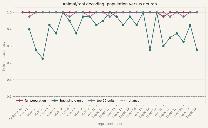
The third experiment asked whether a simple classifier could recover the categories from these activations. This is called a linear probe. The language model stays frozen. The probe only learns a weighted vote: which recorded activations, added together, best separate animals from tools?
The animal/tool test was easy enough that a single unit, a group of units, and the full input embedding could all reach 100% on the small held-out set. That is a ceiling effect. Accuracy has run out of room to tell these representations apart.
Remove the obvious word
The next experiment removed the easiest clue: the animal or tool word itself. Each of 60 concepts appeared in three forms. For a baboon, the model saw:
LiteralA baboon was described. They then referred to this entity
DescriptionA large social primate with a dog-like muzzle and expressive face was described. They then referred to this entity
ContextAt the rocky troop’s edge, it watched for danger while others searched the ground. They then referred to this entity
I recorded the activation at the final word, entity. That word was identical in all 180 prompts. A category difference there must come from the preceding sentence, although the sentence can still contain clues such as primate, muzzle, or troop.
The original frozen units transferred less cleanly. Their median effect fell from 3.55 on the first localizer to 1.21 for literal mentions, 1.51 for descriptions, and 0.88 for contexts. Fourteen of the 20 units had positive effects in each form.
Population probes did better. In five folds that kept all forms of a concept together, a probe trained on literal forms reached 100% on descriptions and 93.3% on contexts at layer 4. These are the best observed layer results in that evaluation. They show useful transfer across forms; they do not establish a uniquely abstract layer.
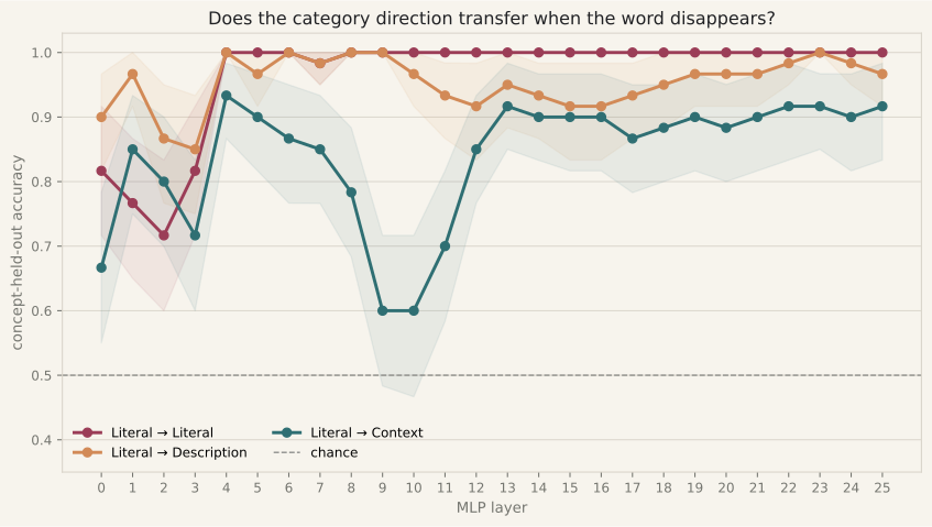
This is the difference between asking whether one knob still behaves the same and asking whether the whole control panel still contains usable information. The first answer weakened. The second remained strong.
The attractive story that did not work
Vision offers an attractive picture of depth. Early cells can respond to small spots or oriented edges. Later responses can combine simpler signals into shapes and objects. The classic simple-to-complex hierarchy is not the whole story of vision, but it suggests a powerful question: can basic building blocks become more stable and more concept-like as information moves through a system? Priebe and Ferster (2012).
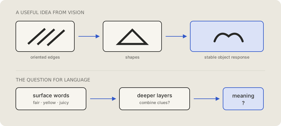
Could language behave in the same way? Early layers might preserve obvious wording. Later layers might combine those clues into meanings that survive paraphrase. If that analogy holds, a concrete thing such as lemon should become recognizable early, while an abstract idea such as justice might need more transformation and peak later.
The fifth experiment used 300 concepts, each with four differently worded descriptions. Human ratings placed every concept on a scale from 1, abstract, to 5, concrete. The ratings came from Brysbaert, Warriner, and Kuperman (2014). The descriptions did not contain the concept name, and each ended with the same neutral anchor word, entity.
Justice · 1.45A subject or item characterized as the quality of being just or fair. They then referred to this entity
Lemon · 5.00A subject or item characterized as yellow oval fruit with juicy acidic flesh. They then referred to this entity
I began with a short preliminary test: could a linear predictor recover the human rating from the 6,912 activations in one layer? On unseen concepts written in a held-out description style, the validation-selected layer reached a correlation of 0.292, while a TF-IDF baseline based only on words and their frequencies reached 0.654. The activations contained some usable information, but this was not a clean abstraction scale.
The more direct test asked a different question: if the model reads two descriptions of the same concept, can it recognize that they refer to the same thing?
Take justice. I used one description as a query, then compared its 6,912-number activation pattern with 60 descriptions written in another style. One candidate also described justice. The other 59 described concepts with similar concreteness ratings. I measured the cosine similarity between the query and every candidate, then ranked the candidates from most to least similar.
QueryA subject or item characterized as the quality of being just or fair. They then referred to this entity
Compare60 descriptions in another writing style: one about justice and 59 about other similarly abstract concepts.
RankWhere does the other justice description appear when activation patterns are ordered by similarity?
The score was mean reciprocal rank, or MRR. If the correct description ranked first, it scored 1. If it ranked second, it scored 1/2; if it ranked tenth, 1/10. Random ranking among 60 candidates would average about 0.078. I repeated the comparison across all pairs of writing styles and in both directions.
I divided the concepts into five equally sized groups, from the most abstract to the most concrete. These are five groups within this dataset, not five equal intervals on the original 1–5 rating scale. The prediction was about where each curve would peak: concrete concepts should peak early, while abstract concepts should shift to the right and peak in later layers.
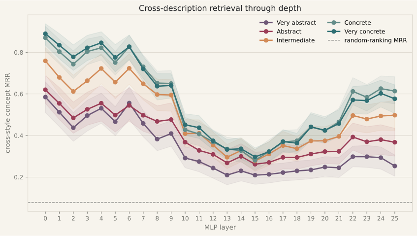
That is not what happened. All five groups reached their best matching score at layer 0, the first MLP block I measured. The very abstract group peaked at 0.585; the very concrete group peaked at 0.890. Concrete concepts were easier to match, but easier is not the same as earlier. The important result is horizontal: none of the abstract groups moved its peak toward deeper layers. Every group also reached 80% of its own best score at layer 0.
A TF-IDF baseline slightly exceeded the best transformer score in all five groups. This suggests that shared words and phrases could solve part of the task. It does not prove that the model lacked concept information, but it limits how much the retrieval scores can tell us about abstraction.
Model scale may be part of the explanation. Anthropic’s Verbalizable Representations Form a Global Workspace in Language Models identifies a small, Jacobian-derived set of directions in large Claude models called the J-space. These directions can carry concepts that the model can report and use flexibly, while much automatic processing happens outside that workspace. The researchers explicitly leave open whether smaller models have an equally rich workspace, a weaker one, or none at all. Gemma 3 1B may therefore be too small for a workspace-like depth effect to appear clearly. But this experiment cannot separate that possibility from a measurement problem: Anthropic studied residual-stream directions and tested them with interventions, while I compared all gated MLP activations. A useful follow-up would repeat this test across model sizes with a J-lens-like measurement.
Layer 0 is also not a raw word embedding. It is the first contextual MLP block, after attention has already processed the description. The result therefore does not say that abstraction exists before contextual processing. It says that different descriptions were already highly matchable at the earliest internal point I measured.
So the attractive story did not survive this test. Abstract concepts were harder to match than concrete ones, but they did not emerge later. This model, these descriptions, this readout, and this similarity measure did not reveal the neat progression we expected.
So, did we find an animal neuron?
We found units with large, repeatable animal-versus-tool differences. Most of the selected units preferred animals across a wider category set; a few preferred plants or food. Some category information transferred when we changed the wording and measured a shared token.
Those are useful observations. They do not show that one unit is a concept, that the model needs it to recognize animals, or that changing it would produce a predictable change in an answer. These experiments record activations and fit probes. They do not disable units or intervene on the model’s computation.
For me, the psychology connection is most useful here. The work is in turning an appealing label into a sequence of contrasts. What else could explain the response? Which examples were used to select it? Does the pattern survive a different question?
I would follow this with better-matched vocabulary, more varied descriptions, and a controlled intervention on selected units. Each would test a different gap. The current study stops before those claims.
For now, try a smaller experiment yourself: open Neural Observatory, choose a unit, and predict its strongest category before looking at the individual words. Then change the layer or choose another unit. The point is to see how much a response can tell us—and how quickly a name can outrun it.
Measurements and source records
All model results above come from saved runs of google/gemma-3-1b-pt, revision fcf18a2a879aab110ca39f8bffbccd5d49d8eb29. Layer IDs are zero-based. The first three experiments use curated single-token words; the later experiments use a shared contextual anchor. The browser playground displays saved activations and does not run the model or change its weights.
The downloadable evidence snapshot contains the first four experiment summaries and the tables behind the fifth experiment’s comparisons. It includes source paths and the model revision. These are exploratory results from one model, not a general map of language-model cognition.